What’s Cooking?

Predicting recipe cuisine from a “bag-of-ingredients” model

This is an old Kaggle competition that I’ve selected to get more practice with the applied machine learning process, with an emphasis on feature extraction and model selection. The goal of this project is to classify recipes into cuisines using their ingredients. I explored a few common classifiers, such as Naive Bayes and Random Forests, and evaluated their performance on this data set to see what the best classifier for this data would be.

Data

I pulled this data, provided by Yummly for the competition, from Kaggle’s API. The data is in unnormalized form and stored in JSON format with recipe id, the type of cuisine, and the variable length list of ingredients of each recipe. The training set and test set are identical except that the test set does not have a cuisine label for competition evaluation purposes.

Example Data:

{
 "id": 24717,
 "cuisine": "indian",
 "ingredients": [
     "tumeric",
     "vegetable stock",
     "tomatoes",
     "garam masala",
     "naan",
     "red lentils",
     "red chili peppers",
     "onions",
     "spinach",
     "sweet potatoes"
 ]
 }

Data Load and Exploration

First, I set up my environment.

# imports
import json
import re
import warnings

import matplotlib.pyplot as plt
import numpy as np
import pandas as pd
import seaborn as sns

from sklearn.dummy import DummyClassifier
from sklearn.ensemble import RandomForestClassifier, GradientBoostingClassifier
from sklearn.feature_extraction.text import CountVectorizer
from sklearn.metrics import f1_score, accuracy_score, confusion_matrix, classification_report
from sklearn.model_selection import train_test_split, cross_val_score
from sklearn.naive_bayes import MultinomialNB
from sklearn.neighbors import KNeighborsClassifier
from sklearn.tree import DecisionTreeClassifier

# set plot style to Seaborn
sns.set_style("white")
sns.set_style("ticks")
sns.set(font_scale=1.5)

# Filter out FutureWarnings from model evaluation
warnings.filterwarnings('ignore')

%matplotlib inline

Next, I load the data into my environment and print out the first value from each data set to ensure it loaded in as expected. I already saved down the data from Kaggle as JSON files in the same directory as this notebook on my computer.

def load_data(directory):
    """Load in recipe data as list of dicts

    Args:
        directory (str): absolute filepath where train and test data can be found

    Returns:
        A list of dicts representing the training data possessing a 'cuisine' label
        and a list of dicts representing the test data without a 'cuisine' label
    """
    with open(f'{directory}/train.json', 'r') as file:
        train_data = json.load(file)

    with open(f'{directory}/test.json', 'r') as file:
        test_data = json.load(file)

    return train_data, test_data

train_data, test_data = load_data('~/Desktop/W207')
print(len(train_data))
print(train_data[0])
print(test_data[0])

39774
{'id': 10259, 'cuisine': 'greek', 'ingredients': ['romaine lettuce', 'black olives', 'grape tomatoes', 'garlic', 'pepper', 'purple onion', 'seasoning', 'garbanzo beans', 'feta cheese crumbles']}
{'id': 18009, 'ingredients': ['baking powder', 'eggs', 'all-purpose flour', 'raisins', 'milk', 'white sugar']}

The training data point has id, cuisine, and ingredients keys and the test data only has id and ingredients keys as expected.

Before jumping into data preprocessing, it’s important to explore the classes and features to get a sense for what machine learning approach to take. I examined class distribution, to determine whether or not I was dealing with significant class imbalance, as well as feature distribution, to determine the sparsity of the data.

First, I examined class distribution by grouping recipe counts by cuisine.

def class_distribution(train_data):
    """Plot a bar chart of the distribution of class labels
    in the recipe train data. Find the frequencies of the most
    and least prevalent class labels and compute their ratio.

    Args:
        train_data (list of dicts): train data possessing a "cuisine" key

    Returns:
        A tuple of the label and count for the most frequent class and
        a tuple of the label and count for the least frequent class.
    """
    cuisine_labels = [datum['cuisine'] for datum in train_data]
    label_table = pd.DataFrame(data=cuisine_labels, columns=['Cuisine'])
    print(f'Number of classes: {len(np.unique(cuisine_labels))}')

    plt.figure(figsize=(16,10))
    sns.countplot(x=label_table.columns[0], data=label_table)
    sns.despine()
    plt.xticks(rotation=-45)

    frequency = label_table.groupby('Cuisine').size()

    most_frequent = (frequency.idxmax(), frequency.max())
    least_frequent = (frequency.idxmin(), frequency.min())

    return most_frequent, least_frequent

most_frequent, least_frequent = class_distribution(train_data)
print(f'Most Frequent Class: {most_frequent[0]} - {most_frequent[1]}')
print(f'Least Frequent Class: {least_frequent[0]} - {least_frequent[1]}')
print(f'Class Imbalance: {most_frequent[1] / least_frequent[1]:.1f}')

Number of classes: 20
Most Frequent Class: italian - 7838
Least Frequent Class: brazilian - 467
Class Imbalance: 16.8

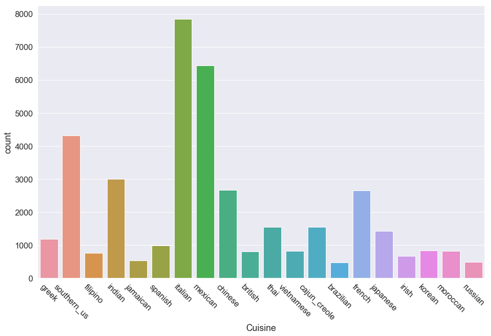
The three predominant classes are italian, mexican and southern_us. I measured class imbalance as the ratio between the most and least prevalent classes and noted there are 16 times more italian recipes than brazilian recipes. The frequency plot also shows that around 9-12 other cuisines have frequencies similar to brazilian indicating this data set has a sever class imbalance. There are two key takeaways from this:

• Most machine learning classifiers will tend to overfit to our top three cuisines
• Accuracy alone may not be an adequate metric for evaluating classifiers

Another indicator of data distribution I chose to explore was the number of unique features per class. While any bag-of-words model will be very sparse, I felt it was reasonable to assume that there were many recipes that shared common ingredients within and between cuisines.

def unique_features(train_data):
    """Plot a bar chart of the distribution of unique features
    in the recipe train data. Find the feature counts of class labels
    with the most and least number of unique features and compute the ratio.

    Args:
        train_data (list of dicts): train data possessing a "cuisine" key

    Returns:
        A tuple of the label and count for the class with most features and
        a tuple of the label and count for the class with least features.
    """
    cuisines = set([datum['cuisine'] for datum in train_data])
    recipes = dict(zip(cuisines, [list() for x in cuisines]))

    for cuisine in recipes.keys():
        [recipes[cuisine].extend(datum['ingredients']) for datum in train_data if datum['cuisine'] == cuisine]
        recipes[cuisine] = len(set(recipes[cuisine]))

    recipe_table = pd.DataFrame.from_dict(data=recipes, orient='index', columns=['UniqueCount'])

    plt.figure(figsize=(16,10))
    sns.barplot(x=recipe_table.index, y='UniqueCount', data=recipe_table)
    sns.despine()
    plt.xticks(rotation=-45)

    most_features = (recipe_table.idxmax().values[0], recipe_table.max().values[0])
    least_features = (recipe_table.idxmin().values[0], recipe_table.min().values[0])

    return most_features, least_features

most_features, least_features = unique_features(train_data)
print(f'Class with Most Features: {most_features[0]} - {most_features[1]}')
print(f'Class with Least Features: {least_features[0]} - {least_features[1]}')
print(f'Feature imbalance: {most_features[1] / least_features[1]:.1f}')

Class with Most Features: italian - 2929
Class with Least Features: brazilian - 853
Feature imbalance: 3.4

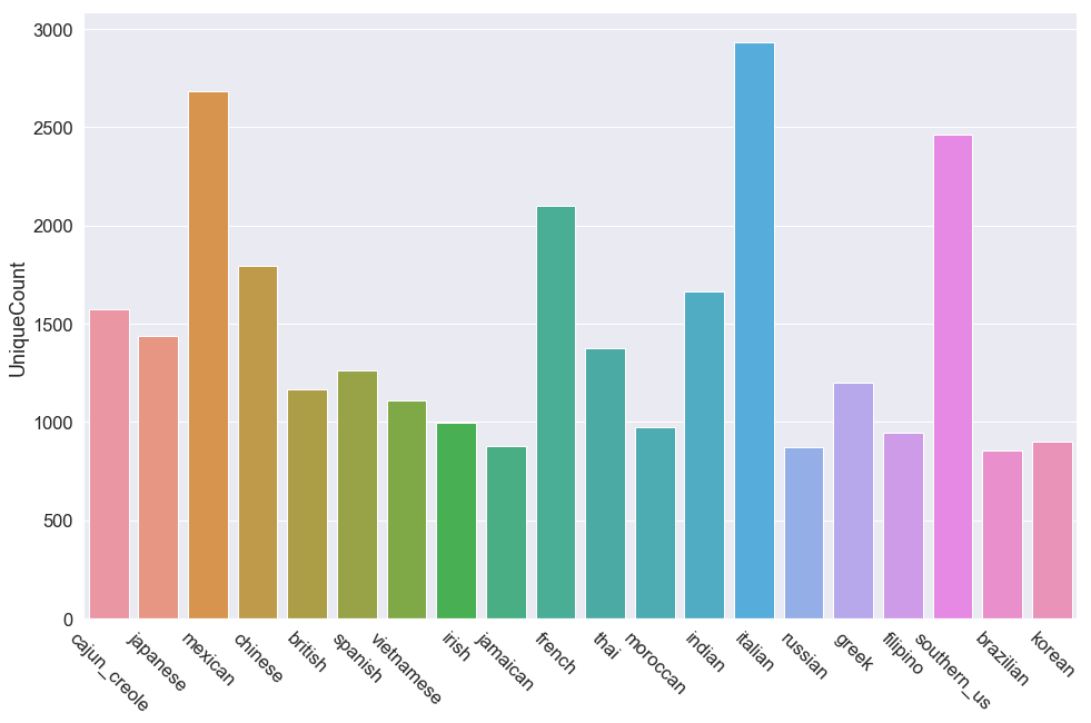
The frequency plot shows feature diversity is much more uniformly spread than class diversity. A unique feature imbalance of 3x is nowhere near as concerning as a class imbalance of 16x; in addition, the feature imbalance may be influenced by the class imbalance itself. I don’t note any particular concerns from this attribute.

The last distribution I examined was the average number of features per class, or in this case, the average number of ingredients per recipe for each cuisine.

def avg_features(train_data):
    """Plot a bar chart of the distribution of average count of features
    in the recipe train data. Find the average feature counts of class labels
    with the most and least number of average features and compute the ratio.

    Args:
        train_data (list of dicts): train data possessing a "cuisine" key

    Returns:
        A tuple of the label and count for the class with most average features and
        a tuple of the label and count for the class with least average features.
    """
    cuisines = set([datum['cuisine'] for datum in train_data])
    recipes = dict(zip(cuisines, [list() for x in cuisines]))
    error = dict.fromkeys(cuisines)

    for cuisine in recipes.keys():
        [recipes[cuisine].append(len(datum['ingredients'])) for datum in train_data if datum['cuisine'] == cuisine]
        error[cuisine] = np.std(recipes[cuisine])
        recipes[cuisine] = np.mean(recipes[cuisine])

    recipe_table = pd.DataFrame.from_dict(data=recipes, orient='index', columns=['AvgFeatures'])
    recipe_table["Error"] = pd.Series(error)

    plt.figure(figsize=(16,10))
    x = recipe_table.index.values
    y = recipe_table.AvgFeatures.values
    err = recipe_table.Error.values
    sns.barplot(x=x, y=y, yerr=err, data=recipe_table)
    sns.despine()
    plt.xticks(rotation=-45)

    most_avg_features = (recipe_table.AvgFeatures.idxmax(), recipe_table.AvgFeatures.max())
    least_avg_features = (recipe_table.AvgFeatures.idxmin(), recipe_table.AvgFeatures.min())

    return most_avg_features, least_avg_features

most_avg_features, least_avg_features = avg_features(train_data)
print(f'Class with Most Average Features: {most_avg_features[0]} - {most_avg_features[1]}')
print(f'Class with Least Average Features: {least_avg_features[0]} - {least_avg_features[1]}')
print(f'Average feature imbalance: {most_avg_features[1] / least_avg_features[1]:.1f}')

Class with Most Average Features: moroccan - 12.909866017052375
Class with Least Average Features: irish - 9.299850074962519
Average feature imbalance: 1.4

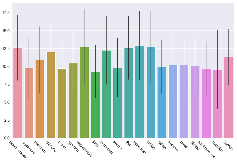
This frequency plot shows the most uniform distribution I’ve seen yet. Given the class imbalance I observed earlier, it is a pretty good sign that the average number of features per class are relatively close. I think it is safe to proceed with using machine learning classifiers to predict on this dat set.

Data Preprocessing

As this text data is in unnormalized form, I suspect there may be some ingredients with special characters.

def get_special_chars(regex, features):
    """Uses regex to find special characters in a list of text features

    Args:
        regex (str): a string containing a regex expression for matching
        features (list of str): a list containing non-unique text features
        special_chars (dict)

    Returns:
        A list of strings containing unique text features
        containing specified special chars.
    """
    special_chars = []

    for f in features:
        if re.match(regex, f) and f not in special_chars:
            special_chars.append(f)

    return special_chars


def search_special_chars(train_data, test_data):
    """Search for special characters within the feature set of ingredients

    Args:
        train_data (list of dicts): train data possessing a "cuisine" label
        test_data (list of dicts): test data without a "cuisine" label

    Returns:
        A dictionary mapping strings representing train/test to a list of
        strings containing text features with special characters in them.
    """
    train_ingredients, test_ingredients = [], []
    [train_ingredients.extend(datum['ingredients']) for datum in train_data]
    [test_ingredients.extend(datum['ingredients']) for datum in test_data]

    regex = '\(|@|\$\?'
    special_chars = {}
    special_chars['train'] = get_special_chars(regex, train_ingredients)
    special_chars['test'] = get_special_chars(regex, test_ingredients)

    return special_chars

special_chars = search_special_chars(train_data, test_data)
print(f'Training features with special characters: {special_chars["train"]}')
print(f'Training features with special characters: {special_chars["test"]}')

Training features with special characters: ['(    oz.) tomato sauce', '(10 oz.) frozen chopped spinach, thawed and squeezed dry', '(   oz.) tomato paste', '(14.5 oz.) diced tomatoes', '(15 oz.) refried beans', '(10 oz.) frozen chopped spinach', '(14 oz.) sweetened condensed milk']
Training features with special characters: ['(    oz.) tomato sauce', '(14.5 oz.) diced tomatoes']

There aren’t too many features with special characters, however, I noticed there are measurement amounts in some of the ingredients. While there may be some information in ingredient measurement (perhaps italian cuisine uses more tomatoes than greek cuisine, despite them both using tomatoes), there could be confusion created between recipes using different measurements within a cuisine.

def search_numeric_chars(train_data, test_data):
    """Search for numeric characters within the feature set of ingredients

    Args:
        train_data (list of dicts): train data possessing a "cuisine" label
        test_data (list of dicts): test data without a "cuisine" label

    Returns:
        A dictionary mapping strings representing train/test to a list of
        strings containing text features with special characters in them.
    """
    train_ingredients, test_ingredients = [], []
    [train_ingredients.extend(datum['ingredients']) for datum in train_data]
    [test_ingredients.extend(datum['ingredients']) for datum in test_data]

    regex = '\S*\d+\S*'
    numeric_chars = {}
    numeric_chars['train'] = get_special_chars(regex, train_ingredients)
    numeric_chars['test'] = get_special_chars(regex, test_ingredients)

    return numeric_chars

numeric_chars = search_numeric_chars(train_data, test_data)
print(f'Training features with numeric characters: {len(numeric_chars["train"])}\n{numeric_chars["train"]}')
print(f'Training features with numeric characters: {len(numeric_chars["test"])}\n{numeric_chars["test"]}')

Training features with numeric characters: 27
['1% low-fat milk', '2% reduced-fat milk', '1% low-fat cottage cheese', '(10 oz.) frozen chopped spinach, thawed and squeezed dry', '1% low-fat buttermilk', '95% lean ground beef', '(14.5 oz.) diced tomatoes', '1% low-fat chocolate milk', '7 Up', '40% less sodium taco seasoning', '2% low-fat cottage cheese', '8 ounc ziti pasta, cook and drain', '25% less sodium chicken broth', '33% less sodium cooked ham', '(15 oz.) refried beans', '(10 oz.) frozen chopped spinach', '33% less sodium ham', '40% less sodium taco seasoning mix', '(14 oz.) sweetened condensed milk', '33% less sodium smoked fully cooked ham', 'v8', '2% low fat cheddar chees', 'V8 Juice', '2% lowfat greek yogurt', '33% less sodium cooked deli ham', '2 1/2 to 3 lb. chicken, cut into serving pieces', '2% milk shredded mozzarella cheese']
Training features with numeric characters: 16
['1% low-fat cottage cheese', '2% reduced-fat milk', '7 Up', '95% lean ground beef', '1% low-fat milk', '33% less sodium smoked ham', 'V8 100% Vegetable Juice', '1% low-fat buttermilk', '33% less sodium cooked deli ham', '(14.5 oz.) diced tomatoes', '2% low-fat cottage cheese', '8 ounc ziti pasta, cook and drain', '2% reduced fat chocolate milk', '2% lowfat greek yogurt', '40% less sodium taco seasoning', '50% less sodium black beans']

While this may be an issue, there are only 27 data points in the training set that have numbers in them. I decide this is not enough to be worth the preprocessing step and proceed with feature extraction.

def extract_text_features(train_data, num_examples=5):
    """Extracts text features from list of ingredients and prints a few examples

    Args:
        train_data (list of dicts): train data possessing a "cuisine" label
        num_examples: The number of examples to be printed

    Returns:
        A Compressed Sparse Row matrix object containing the extracted text features
    """
    feature_separator = '|'
    feature_decoder = r'\|([a-zA-z ]*)\|'
    train_features = np.array([feature_separator.join(datum['ingredients']) for datum in train_data])
    vectorizer = CountVectorizer(token_pattern=feature_decoder)
    train_features = vectorizer.fit_transform(train_features)
    feature_names = vectorizer.get_feature_names()

    for i in range(num_examples):
        example_feature = feature_names[np.random.randint(0, train_features.shape[1])]
        print(f'Example feature {i + 1}: {example_feature}')

    return train_features

def examine_csr_matrix(csr_matrix):
    """Examines some key features of a csr matrix to confirm feature extraction
    succeeded

    Args:
        csr_matrix (scipy.sparse.csr_matrix): Compressed Sparse Row matrix object
        containing extracted text features
    """
    # examine size of vocabulary
    print(f'Size of feature vocabulary: {csr_matrix.shape[1]}')

    # examine average number of nonzero features per datum
    nnz = [datum.nnz for datum in csr_matrix]
    average_nnz = sum(nnz) / len(nnz)
    print(f'Average non-zero features: {average_nnz: .2f}')

    # examine fraction of non-zero entires
    frac_nnz = sum(nnz) / (csr_matrix.shape[0] * csr_matrix.shape[1])
    print(f'Fraction of non-zero entries: {frac_nnz: .6f}')

def process_labels(train_data):
    """Extracts class labels from the training data

    Args:
        train_data (list of dicts): train data possessing a "cuisine" label

    Returns:
        A numpy array containing the class labels as strings
    """
    return np.array([datum['cuisine'].strip() for datum in train_data])

train_features = extract_text_features(train_data)
train_labels = process_labels(train_data)
examine_csr_matrix(train_features)

Example feature 1: gumbo file
Example feature 2: boar
Example feature 3: grapefruit juice
Example feature 4: collard green leaves
Example feature 5: fillet steaks
Size of feature vocabulary: 4958
Average non-zero features:  4.56
Fraction of non-zero entries:  0.000919

Looking good! I note that the feature vocabulary size is very small, a little less than 5000 ingredients, with an average of 4.5 ingredients per recipe. This may be difficult for a classifier to pick up on patterns, so I’m expecting an overall poor performance with a CountVectorizer matrix.

Model Selection

Now that our features are vectorized, they can be passed into classifiers. From the data exploration section, I decided to not rely solely on accuracy as an evaluation metric, so I will be using accuracy and F1 score to get a sense of performance on both precision and recall. Before I begin the model seleciton process, I need to establish a baseline to compare to. Two common baselines are random selections from a uniform distribution $\frac{1}{20}$ or $0.05$ or always guessing the most common classifier $\frac{7838}{39774}$ or $0.197$. I use sckit-learn’s DummyClassifier class to evaluate a couple of common baselines and select the one I’ll be using for the rest of the model selection process.

I also build out some helper functions that will give me a good high-level summary of each model I’m testing.

from sklearn.dummy import DummyClassifier

def print_header(content):
    """Prints a nicely formatted header describing the intention of a metric"""
    print('-'*100)
    print(content)
    print('-'*100)

def plot_scores(scores):
    """Plots the distribution of generated metrics from a classifier using cross_val_score

    Args:
        scores (tuple of np.ndarray of float): Accuracy and f1 scores to be plotted
    """
    f, axes = plt.subplots(1, 2, figsize=(16, 10), sharex=True)
    sns.despine()
    sns.distplot(scores[0], kde=False, rug=True, ax=axes[0]).set_title('Accuracies')
    sns.distplot(scores[1], kde=False, rug=True, ax=axes[1]).set_title('F1 Scores')

def plot_confusion_matrix(cm, class_names):
    """ Plots a normalized lower triangular confusion_matrix (due to class imbalance) to visualize performance
    of classifier's predictions

    Args:
        cm (confusion_matrix): A confusion matrix for a classifier's predictions
        class_names (np.ndarray of str): An array of class names for axes
    """
    cm = cm.astype('float') / cm.sum(axis=1)[:, np.newaxis]
    plt.figure(figsize=(16,10))
    mask = np.zeros_like(cm)
    mask[np.triu_indices_from(mask)] = True
    with sns.axes_style("white"):
        sns.heatmap(cm,
                    xticklabels=class_names,
                    yticklabels=class_names,
                    mask=mask, linewidths=.25, cmap="gray_r")

def baseline_scores(train_features, train_labels, train_size=0.8):
    """Uses a DummyClassifier to produce the best baseline value for evaluating model performance

    Args:
        train_features (scipy.sparse.csr_matrix): Contains the extracted training text features
        train_labels (np.ndarray of str): Contains the class labels
        train_size (float): The proportion of the data to be split into a training set

    Returns:
        A tuple pairing the classifier name to the best baseline score for a DummyClassifier
    """
    X_train, X_test, y_train, y_test = train_test_split(train_features, train_labels, train_size=train_size)
    strategies = ['stratified', 'most_frequent', 'prior', 'uniform']
    baseline = [DummyClassifier(strategy=strategy, random_state=42).fit(X_train, y_train).score(X_test, y_test)
                for strategy in strategies]
    baseline = ('dummy', max(baseline))
    return baseline


def examine_classifier(clf, clf_name, train_features, train_labels, baseline, train_size=0.8, report=None):
    """Train and evaluate a single iteration of a classifier to get a sense of how it performs on data

    Args:
        clf (sklearn classifier object): The classifier to be examined
        clf_name (str): The name of the classifier being examined
        train_features (scipy.sparse.csr_matrix): Contains the extracted training text features
        train_labels (np.ndarray of str): Contains the class labels
        baseline (tuple): The classifier name and baseline to beat
        train_size (float): The proportion of the data to be split into a training set
        additional (None or str): If 'report', print out a classification report. If 'matrix',
        plot a heatmap on a confusion matrix
    """
    print_header(f'Examining {clf_name} performance on recipe data')
    X_train, X_test, y_train, y_test = train_test_split(train_features, train_labels, train_size=train_size)
    clf.fit(X_train, y_train)
    y_predict = clf.predict(X_test)

    accuracy = accuracy_score(y_test, y_predict)
    f1 = f1_score(y_test, y_predict, average='weighted')
    print(f'Accuracy {accuracy:.6f} compared to best classifier {baseline[0]} baseline score of {baseline[1]:.6f}')
    print(f'Difference: {((accuracy - baseline[1]) / baseline[1]) * 100:.2f}%\n')

    print(f'F1 Score {f1:.6f} compared to best classifier {baseline[0]} baseline score of {baseline[1]:.6f}')
    print(f'Difference: {((f1 - baseline[1]) / baseline[1]) * 100:.2f}%\n')

    if report == 'report':
        print_header(f'Classification Report for {clf_name}')
        print(classification_report(y_test, y_predict))
    elif report == 'matrix':
        print_header(f'Confusion Matrix for {clf_name}')
        class_names = clf.classes_
        plot_confusion_matrix(confusion_matrix(y_test, y_predict), class_names)


def evaluate_classifier(clf, clf_name, train_features, train_labels, baseline, cv=100, score_dist=False):
    """Train and evaluate multiple iterations of a classifier to get overall performance and update baseline

    Args:
        clf (sklearn classifier object): The classifier to be evaluated
        clf_name (str): The name of the classifier being evaluated
        train_features (scipy.sparse.csr_matrix): Contains the extracted training text features
        train_labels (np.ndarray): Contains the class labels
        baseline (tuple): The classifier name and baseline to beat
        cv (int): The number of folds to be used in a stratified K-Fold
        score_dist (bool): If True, plot the distribution of accuracies and f1 scores for this classifier

    Returns:
        A tuple that either is the old baseline if it is not beat or this classifiers average f1 score if it is
    """
    print_header(f'Evaluating {clf_name} performance on recipe data')
    accuracies = cross_val_score(clf, train_features, train_labels, scoring='accuracy', cv=cv)
    f1_scores = cross_val_score(clf, train_features, train_labels, scoring='f1_weighted', cv=cv)

    if score_dist:
        print_header(f'Score distributions for {clf_name}')
        plot_scores((accuracies, f1_scores))

    avg_accuracy = np.mean(accuracies)
    avg_f1_score = np.mean(f1_scores)

    if avg_f1_score < baseline[1] < avg_accuracy:
        print(f'{clf_name} average accuracy beats baseline BUT f1_score does not THEREFORE will not update baseline')
    elif avg_f1_score > baseline[1]:
        print(f'{clf_name} average f1_score beats baseline THEREFORE updating baseline\nGain of {((avg_f1_score - baseline[1]) / baseline[1]) * 100:.2f}%')
        baseline = (clf_name, avg_f1_score)
    else:
        print(f'{clf_name} average accuracy and f1_score both do not beat baseline THEREFORE will not update baseline')

    return baseline

baseline = baseline_scores(train_features, train_labels)

Now that I have a baseline selected, I can proceed with testing out a few classifiers!

My first intuition is to use a Multinomial Naive Bayes classifier, which is a common classifier used to evaluate text data.

examine_classifier(MultinomialNB(), 'Multinomial Naive Bayes', train_features, train_labels, baseline, report='matrix')

----------------------------------------------------------------------------------------------------
Examining Multinomial Naive Bayes performance on recipe data
----------------------------------------------------------------------------------------------------
Accuracy 0.592332 compared to best classifier dummy baseline score of 0.200503
Difference: 195.42%

F1 Score 0.553125 compared to best classifier dummy baseline score of 0.200503
Difference: 175.87%

----------------------------------------------------------------------------------------------------
Confusion Matrix for Multinomial Naive Bayes
----------------------------------------------------------------------------------------------------

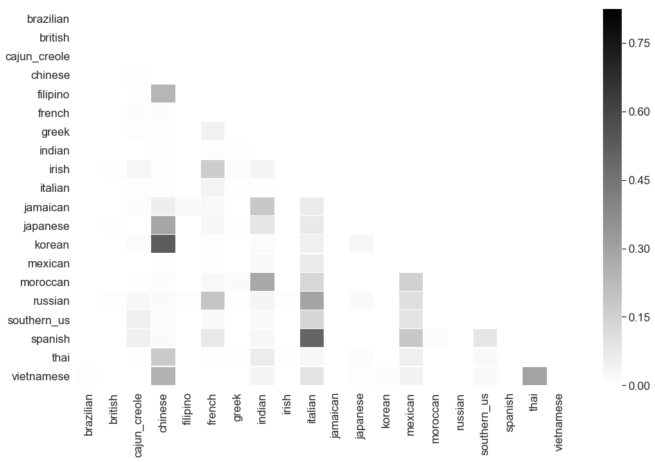
Not great. A performance of $0.55$ is not fantastic, but it does better than the baseline of always guessing italian. The Multinomial Naive Bayes confusion matrix also shows that most of the predictions are ending up in our dominant classes; our class imbalance is really having an impact on our results.

An interesting behavior: many Asian cuisines (Korean, Japanese, Thai, Vietnamese, Filipino) end up in the Chinese class. This leads me to wonder if shared ingredients by geographic region is confusing the Multinomial Naive Bayes model. As Naive Bayes is a probability based model, the more shared features among classes, the less sure it will be in predicting the cuisine of a class. For example, if the probability of soy sauce appearing in Japanese, Chinese, or Thai recipes is $0.33$, a Naive Bayes model will split it amongst those three classes. Not quite the best approach when predicting cuisine.

Another popular classifiers to use are Random forests, or an ensemble of decision trees.

examine_classifier(RandomForestClassifier(), 'Random forest', train_features, train_labels, baseline, report='matrix')

----------------------------------------------------------------------------------------------------
Examining Random forest performance on recipe data
----------------------------------------------------------------------------------------------------
Accuracy 0.484978 compared to best classifier dummy baseline score of 0.200503
Difference: 141.88%

F1 Score 0.463733 compared to best classifier dummy baseline score of 0.200503
Difference: 131.28%

----------------------------------------------------------------------------------------------------
Confusion Matrix for Random forest
----------------------------------------------------------------------------------------------------

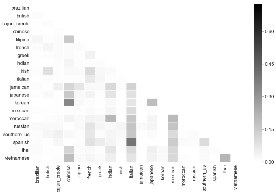
Even worse performance than the Multinomial Naive Bayes model! Let’s try a Gradient Boosted Decision Tree, or an iteration of decision trees where each subsequent tree is weighted to focus on the misclassifications of the previous one.

examine_classifier(GradientBoostingClassifier(), 'GBDT', train_features, train_labels, baseline, report='matrix')

----------------------------------------------------------------------------------------------------
Examining GBDT performance on recipe data
----------------------------------------------------------------------------------------------------
Accuracy 0.529730 compared to best classifier dummy baseline score of 0.200503
Difference: 164.20%

F1 Score 0.510481 compared to best classifier dummy baseline score of 0.200503
Difference: 154.60%

----------------------------------------------------------------------------------------------------
Confusion Matrix for GBDT
----------------------------------------------------------------------------------------------------

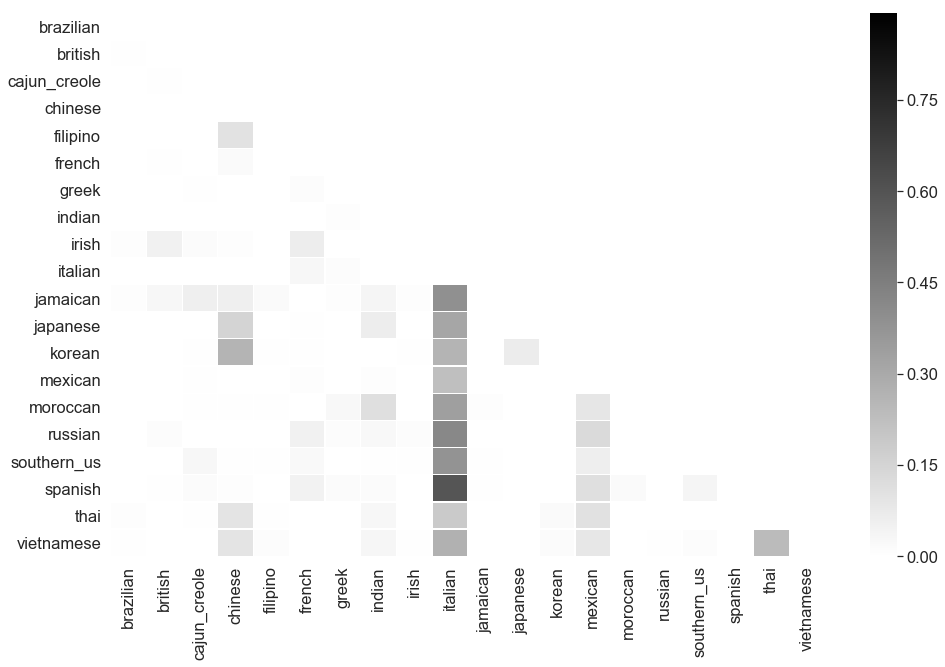
That took a long time and didn’t get much gain either. In fact, it appears there was a further overfit to italian.

Up Next: Neural Networks!

# Neural Networks - in progress